The very first calculation model can be considered the model of the founder of the German Argus pulsejets, Dr. Schulz-Grunow – this is the famous method of characteristics. Those who wish can even familiarize themselves with this method on our website by downloading the corresponding NASA report written by this outstanding scientist. Although this method has its supporters, it was created still in the 40s of the last century for manual calculation and gradually became popular in the modeling of unsteady flows of compressible gas. Unfortunately, for 80 years after its first use, nothing is known about programs for modeling pulsating jet engines based on the method of characteristics and available to a wide range of users.

The same can be said about other methods. A number of well-known scientific works are devoted to thermodynamic models within the framework of the so-called 'piston' analogy of gas movement in a resonant exhaust pipe, when the gas is considered as a 'liquid piston'. One of the founders of this method should be recognized as the Soviet scientist Professor E.S. Shchetinkov, whose developments date back to the 40s of the last century. By the way, a similar principle was later adopted in the study of pulsejets and by other scientists. However, no practically useful models for independent users based on the analogy of the 'liquid piston', and even more so, ready-made programs, have appeared yet.

Methods based on a 1-dimensional representation of gas flow in a resonant pipe are also known. And there are also methods built on the acoustic analogy of oscillations excited in the Helmholtz resonator. But with all these methods there is the same problem again – the average user cannot use these achievements and such advanced models. That is, the user is once again offered to repeat all the calculations of this or that scientist, to create a program himself, to debug it, repeating all the efforts of the author of the model, and only after that to perform the modeling. Who in their right mind and sober memory will repeat all this, when and at whose expense? Answers from scientists have not yet been received...

In the 60-80s of the last century, even the famous professor Gordon Blair from the Belfast Queen's University, recognized authority in modeling of the working process of internal combustion engines (ICE), including racing ones, was involved in developing a model and program for pulsejet engine simulating. Professor Blair even made his own program for simulating pulsejets based on and by analogy with an ICE, including one-dimensional flow of compressed gas through pipes. But the situation repeated: he did not bring the program to commercial use, and it, along with other similar programs, remained inaccessible to a wide range of users.

But the most difficult situation arose with the appearance and widespread introduction of 3-D modeling into scientific practice. Since after purchasing the appropriate program there is no need to invent anything new or your own, some of the most advanced scientists rushed to show in their articles beautiful color pictures of the distribution of gas parameters along the pipe of a pulsejet engine. Others hastened to focus their efforts on the features of modeling 3-dimensional flow with chemical reactions of pulsating combustion, since a good and expensive program allows it. The third, apparently, in the depths of their scientific souls not trusting standard programs, urgently began to develop their own 3-D models of a pulsejet engine, the fourth, on the contrary, after not very successful attempts to create something of their own, returned to standard 3-D programs. True, again with a not entirely clear goal – either to obtain the characteristics that they never obtained or to show other scientists their special knowledge of spatial modeling based on other people's models. The fifth...

It is amazing, but for 80 years thousands of scientists, unknown and known, have studied the pulsejet engine up and down, written thousands of articles, invented hundreds of models for its calculation and even published large books, but for some reason none of them bothered to write a formula for the thrust of this engine. Meanwhile, this is one of the main questions of the theory of jet engines, it is with it that the study of engines begins, and the magnitude of the thrust is not only the main characteristic, but should also be the goal of any study of the engine. Of course, if this engine is intended for an aircraft. However, apparently, this question was not interesting to scientists at all, their work was carried out for some other purpose.

Therefore, it is completely natural that all these deep studies are united by one and the same result – no programs for modeling a pulsejet engine and its characteristics suitable for wide practical application, after such titanic efforts, again did not appear. The user was once again offered to actually buy an expensive 3-D program himself, understand it himself, having undergone appropriate training, then create a model in this program himself, debug it and only after that, to be sure, model his engine. In this case, it is necessary to repeat some steps already performed by this or that scientist and described in his article. But it is simply not possible to repeat all this. Then a reasonable question arises – why should a user spend money on some program, time to study it, create a model, debug it and simulate an engine, if he has a grinder for cutting stainless steel sheets and a welding machine in his garage?

To sum it up, we can say that for 30 years now we have been observing a completely paradoxical situation – scientists cannot and, apparently, do not want to create a normal working model and program for simulating a pulsejet engine for one reason or another, and users cannot and do not want to use what scientists offer them, since it is completely unsuitable for practical use. Moreover, none of the created models are operational due to the lack of ready-made programs, excessive complexity and/or cost, the impossibility of acquiring or for some other reason that prevents its widespread use by an ordinary user. And then there is every reason to assert that no models and programs for calculating the working cycle of a pulsejet engine have actually been created to date.

And this is precisely what determined the goal of our work – creating a mathematical model and a real program for simulating the working cycle of a pulsejet engine specifically for an ordinary user.

How did we do it?

The first thing we paid attention to was the programs for simulating internal combustion engines. These programs have already become standard, and the calculation models that form their basis are implemented as conventional thermodynamic models, in which the gas in the cylinder is considered as a medium with instantaneous parameters uniformly distributed over the volume. At the same time, the gas flow in the pipes adjacent to the cylinder is considered as 1-dimensional, but taking into account the shape (diameter) of these channels and local hydraulic resistances. Well, and of course, one or another combustion model is used, describing the law of heat release in the cylinder after evaporation and ignition of the fuel.

And why can't we do the same for a pulsejet engine? Not only can, but must, since no one wants to do it. No sooner said than done. We took as a basis the thermodynamic model of Professor E.S. Shchetinkov, but significantly reworked it, especially taking into account the reverse flow in the pipe, when cold air enters the pipe and is then pushed out of it. This part of the model is currently based on the ‘liquid’ piston flow model, but we have provided for the possibility of switching to a 1-dimensional gas flow model in the future, after the program is fully debugged, as is done in the known models of internal combustion engines.

But the most interesting thing was discovered later. It turned out that the flow of gas and air in the intake pipe of a valveless pulsejet engine can also be represented as the movement of a ‘liquid’ piston. At least, with the correct mathematical description, the piston analogy allows you to get the same phase delay in air supply compared to the change in pressure in the combustion chamber, like any other method, including the most complex 3-D models. As a result, we managed to create a universal model of both a valved and valveless pulsejet engine, combining these models in one program for the first time.

As a result, our model received the component blocks as below.

1. Thermodynamic model of pressure and temperature changes in the combustion chamber.

If we assume that the instantaneous pressure and temperature are the same for the allocated volume of the combustion chamber, then we can use the equation of the 1st law of thermodynamics written for a cylinder. From which it follows that:

where p is the pressure;

is the enthalpy of the gas; Q is the amount of supplied (+) and/or removed (–) heat; M is the mass of gas in volume V; Cp is the heat capacity of the gas at constant pressure; R is the gas constant.

Let us consider the section of the pulsejet engine cycle when the pressure in the combustion chamber begins to increase due to the supply of heat to the gas as a result of fuel combustion. Taking into account the equation of state of an ideal gas

after some transformations from the equation of the 1st law of thermodynamics, we can obtain an equation for the temperature in the combustion chamber in the form:

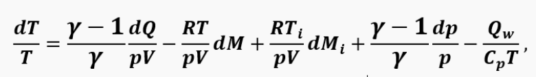
where Q_w is the amount of heat removed to the walls,, γ is heat capacity ratio.

Next, if we differentiate the equation of state of the gas, provided that the volume of the combustion chamber remains constant, we obtain:

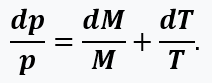
After transformations of both equations, it is easy to obtain a system of 2 differential equations for temperature and pressure, resolved with respect to the derivative, in the form:

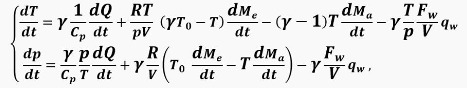
where dMa/dt,dMe/dt are the gas flow rates from the chamber and air flow rates into the chamber, respectively; qw is the specific heat flux into the walls; Fw is the surface area of the walls.

The value of the heat input rate dQ/dt is determined by the selected combustion model. We adopted the following model – heat release is volumetric, that is, it occurs uniformly in the volume of the entire combustion chamber, while the rate of heat release is proportional to the rate of air entering the chamber. That is:

where Hu is the calorific value of the fuel; η is the completeness of combustion, allows us to take into account the influence of the fuel-air mixture composition on the amount of heat released; ρ is the gas density in the chamber; λ is the excess air coefficient; L0 is the stoichiometric ratio.

In reality, heat release does not occur simultaneously with the air intake. On the contrary, at each moment of intake time, only a small portion of air enters the combustion chamber, which is then mixed with the fuel, heated, the fuel evaporates, and only after that this portion of the fuel-air mixture ignites. That is why our model establishes a phase shift in the heat release rate relative to the instantaneous mass flow rate of air. This phase shift is the ignition delay time, which is calculated depending on the pressure and temperature according to the Arrhenius law. However, in relation to our problem, an attempt to directly calculate the ignition delay time gives not quite realistic results, causing instability of the calculation, which is why we switched to relative parameters, but maintaining the general nature of the dependence of time on pressure and temperature. As a result, we obtained the following formula:

where m is a correction factor equal to the fraction of the engine cycle corresponding to the ignition delay at the initial air temperature in the combustion chamber T0 (it is preliminarily assumed that m = 0,3); θ is the ratio of the ignition delay time at temperature T к to the time at temperature T0 (it is preliminarily assumed that θ = 0,1). For combustion completeness, we also approximated the known data and obtained the formula:

where η0 is the maximum coefficient of combustion completeness.

At present, when the work on finalizing the model is not yet finished, heat losses in the walls are temporarily not taken into account when solving the equations for temperature and pressure. Instead, we simply reduce the value of η0, for now, taking it equal to η0 = 0.70-0.75 instead of η0 = 0.95-0.98. Nevertheless, the wall temperature in the model is calculated separately according to the corresponding heat balance equations, taking into account the heat capacity of the walls. This is done due to the discovered problems with the convergence of the solution of the system of differential equations when trying to include the heat flux in the walls in these equations (however, we are working to find and eliminate the cause of such instability).

2. Gas flow through a pipe.

To obtain the calculation equations, we consider a flow with subsonic speeds and pressure differences and assume that the instantaneous pressure, temperature and gas velocity are the same at all points in the pipe. This assumption is applicable for relatively short pipes and reduces the model under consideration to the so-called piston analogy of gas flow, that is, to the model of a 'liquid' or 'gas' piston. Then the movement of gas through the pipe is considered as the movement of a gas column of a certain mass, which has the properties of inertia. This means that under the action of a time-varying pressure difference, the velocity of the gas will lag behind the pressure – approximately the same as when waves move in a pipe.

Calculation scheme of the piston analogy method (‘liquid’ piston): 1 - control volume, 2 - cone (nozzle), 3 - resonance pipe.

Thus, it is obvious that the solution to the problem should be sought in the form of an equation for the velocity of the gas column in the pipe. It is important that the desired velocity is related to the thermodynamic model describing the state of the gas in the control volume to which the pipe is connected. The main calculation equations describing gas-dynamic processes in the pipe in a 1-dimensional approximation are the continuity equation:

and the equation of motion (conservation of momentum):

where t, x are the time and coordinate along the length; p, ρ are the pressure and density of the gas; δ is the fraction of the longitudinal pressure gradient spent on friction and local resistance.

Friction and hydraulic resistance can be taken into account using the total coefficient of hydraulic resistance ξ, then the equation of motion can be represented as:

where ξ=ξ_T+ξ_c, ξ_T=λ_T L⁄D_a is the coefficient of friction losses in the pipe; ξ_c is the coefficient of local resistance at the point of attachment to the volume. The coefficients ξ_T and ξ_c when calculating the flow in the pipe can be found approximately using the formulas used for steady flows.

Let us assume that a gas, located in a control volume under increased pressure, flows through a pipe into the environment. If the equation of motion is multiplied term by term by dx, then due to the adopted assumptions we obtain:

Now we need to integrate the equation from the center of the volume, where we can approximately assume that the gas is motionless, to the pipe exit:

where x_K is the distance from the nozzle exit to the center of the combustion chamber.

After some transformations, we can arrive at the following form of the equation:

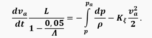
where

and the dimensionless parameter

is the relative volume of the pipe.

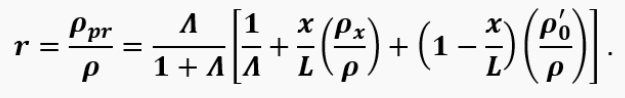
Since the air that was in the pipe at the initial moment of time is quickly pushed out by the gas, which has a higher temperature, we make the assumption that there is no mixing between the gas and air. Then the 'air-gas' boundary will move along the pipe and at some point in time will move away from the beginning of the pipe by a distance x. The pipe contains gases with different densities, so we find some average (reduced) gas density in the form:

where ρ_x is the density of gases in the pipe; ρ_0^' is the density of air in the pipe. If we assume that over a certain period of time ρ_pr is proportional to ρ, i.e.: ρ_pr=rρ , where r=const, then:

The gas densities included in this equation are written using the ideal gas equation as:

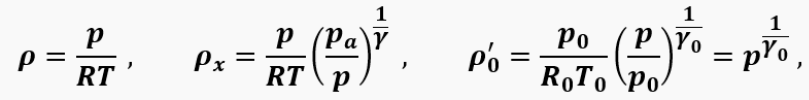
where the parameters with index '0' correspond to the environment. In the absence of heat losses, it can also be assumed that the gas density in the volume depends adiabatically on the pressure. Then the corresponding term in the equation of motion can be represented as:

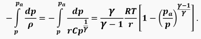
Whence, after the appropriate transformations, we finally obtain for 〖p≥p〗_a and v_a≥0:

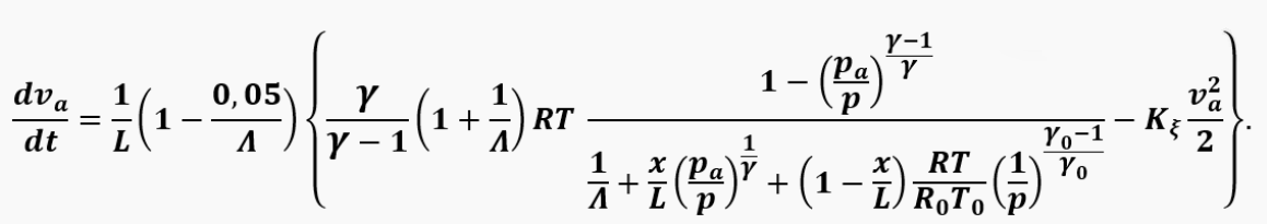
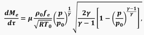
This equation is valid for the positive direction of gas velocity in the pipe when the pressure in the chamber is greater than the static pressure at the pipe exit. Similarly, we can obtain an equation for other conditions of change in the engine cycle, including a negative pressure drop and a negative (towards the combustion chamber) direction of gas movement. Moreover, a completely similar equation can be obtained for the gas/air velocity ve in the intake pipe of a valveless engine if we replace the length L with Le and remove the cone. By the way, knowing the velocity, we can find the instantaneous air flow through the pipe, which is included in the equations for calculating the temperature and pressure in the chamber:

At the same time, attention is drawn to the dependence of gas acceleration on the length of the pipe (the shorter the pipe, the faster the gas accelerates) and on the amount of air in the pipe (the more cold air, the heavier the gas in the pipe and the worse it accelerates). In this case, the air-gas boundary moves along the pipe at a speed of va and can be defined as:

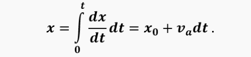
When the coordinate of the boundary x becomes less than zero, this will mean that cold air has begun to enter the chamber. This is the moment used in the model of the intake pipe of a valveless engine as the beginning of intake and a new cycle.

That is, the model as a whole correctly takes into account the features of the real process; at least it provides a qualitative match. From a quantitative point of view, there is a comparison in our articles cited in the 'Library', from which it follows that the discrepancy between the 'liquid' piston model and the one-dimensional model in a fairly wide range of process frequencies is also small. All this allowed us to use this model when writing a program for simulating the working cycle of a pulsejet engine (however, we are already thinking about how to replace this model with a one-dimensional one in the future).

3. Valve system.

For the initial stage of development and operation of the program, we adopted the simplest valve model - quasi-stationary. This is a model that is the simplest and assumes that the frequency of natural oscillations of the petal is many times greater than the frequency of forced oscillations corresponding to the frequency of the engine process. That is, this model does not take into account dynamic phenomena during petal movement. Despite the fact that most scientists are sure that the quasi-stationary model is very bad and wrong, we have previously conducted our own research and compared it with the dynamic one (the corresponding article can be read in our 'Library'). The results were amazing – for the total cyclic air flow rate, and this is the main parameter determining the accuracy of our entire engine model as a whole, the coincidence of the results is no worse than 10-15%.

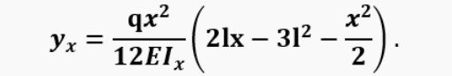
In this case, the inertia of the petal movement and, first of all, its delay when the pressure drop changes can be neglected and the problem can be considered quasi-stationary. For such a problem, obviously, the valve deflection is completely determined by only two factors - the distributed force on the petal (pressure drop Δp) and the valve stiffness. If the valve is a beam rigidly fixed on one side, on which a distributed force q acts, then the dependence of the petal end deflection on this force looks like this:

where E is the elastic modulus of the petal material; I_x is the moment of inertia of the section along the axis; l is the petal length. Considering that I_x=(δ^3 b)⁄(12,) where δ and b are the thickness and width of the petal, and the load on the petal from the pressure drop q=∆pl, it is easy to calculate the dependence of the valve opening (petal deflection) on the pressure drop. All geometric quantities included in these formulas are quite easy to calculate for all selected designs and designs of petal valves.

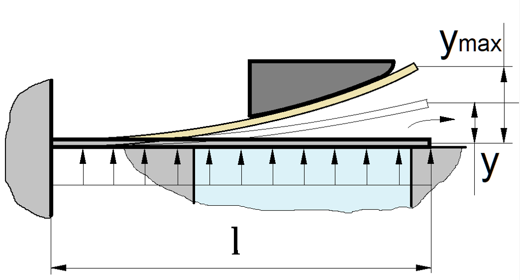
Accepted petal valve design

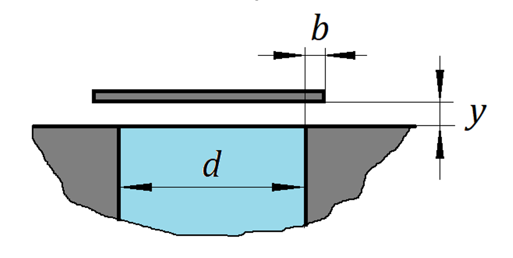
Obviously, to determine the air flow through the valve, it is also necessary to find the hydraulic resistance of the valve. For a plate valve, there is an approximate formula

where y is the valve lift; d is the characteristic diameter of the opening opened by the valve; b is the amount of overlap of the opening by the valve when fully closed.

However, the petal shape affects the opening cross-section for air passage. Therefore, the lift along the petal length x and the area f are found by solving the equation for the petal deflection:

Of course, this simplest model was used only for debugging the program, and we already replaced it with a dynamic one, which we have also already studied in detail (the results are given in the same article). The essence of the valve dynamic model is to numeric solve the differential equation of petal motion with mass and inertia under the action of a variable pressure drop:

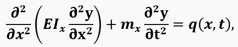
where mx, q(x,t) is the distributed mass and load on the petal from the pressure drop.

This model more accurately reflects the real properties of the petal, including the lag in opening, rebound from extreme positions (you will be able to see this in the calculation results), and, especially, closing lag, when a gases backflow from the combustion chamber appears. Although it also has some shortcomings, which we will gradually eliminate in one way or another in subsequent versions of the program. But we do not plan to deal with it yet 3-D modeling of petal movements with transverse oscillations. In accordance with this, we recommend that all lovers of spatial petal movements in airless space look for other, more accurate online programs and models of pulsejet engines.

Then it only remains to determine the instantaneous air flow through the valve system, which is included in the equations for calculating the temperature and pressure in the chamber:

where

is the flow coefficient, fe is the area opened by all the petals in the valve grid.

In a valveless engine, there are obviously no valves, there the air intake is controlled not by petal valves, but by a pipe with a certain diameter and length (see above).

4. Integration of equations

As a result of all actions, we obtain a system of differential equations describing the working cycle of a pulsejet engine:

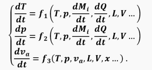
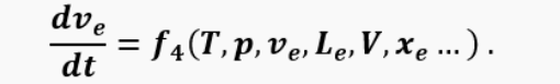
In a valveless engine, one more equation of the form is added to the system:

The solution of the system is performed by the Runge-Kutta method of the 2nd order (modified Euler method). This is a 2-step method, in the first step (half a time step Δt/2) the intermediate value of the function (T, p, v) is calculated:

Then the calculation is carried out first with the new argument of the function, after which in the 2nd step the refined value of the function is calculated

We checked the accuracy of integration in the cycle using the usual 1-step Euler method. It turned out that the 2-step method gives only minor improvements in the accuracy of integration of the cycle parameters, no more than 1-2%. This means that using higher-order methods for our problem simply does not make sense.

Together with the gas parameters, the air and gas mass M, the coordinates of the air-gas boundary in the pipe x and the impulse created by the pipe (in a valveless engine – by two pipes) are integrated. In addition, other auxiliary parameters are calculated in the model, including the adiabatic index and the gas constant of the combustion products from the temperature and composition of the mixture.

5. Calculation of the main engine parameters

The calculation of the main parameters is carried out at the very beginning of the intake: • in a valve engine – when the pressure difference in the chamber changes from positive (above atmospheric) to negative, since the pressure difference determines the intake, • in a valveless engine – when air begins to enter the chamber (the coordinate of the air-gas boundary in the intake pipe becomes less than zero).

The logic of the algorithm determines these moments with high accuracy, and the first thing that is required is to determine the cycle time tc as the time of the start of the intake from a similar previous moment in time. This is a fundamentally important feature of the model - the cycle is not specified in any way, but is determined by the processes that occur in it and are described by the corresponding equations.

Next, after the cycle is completed, the parameters of the cycle themselves are calculated. These include:

cycle frequency:

air and fuel consumption:

where M is the mass of air that passes into the engine per cycle, engine thrust and specific fuel consumption:

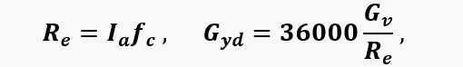
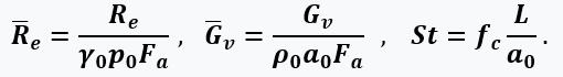
where Ia is the sum (integral) of the instantaneous thrust per cycle, specific thrust, as well as dimensionless thrust, air consumption and cycle frequency (Strouhal number):

For given engine design options and flight mode, it is also possible to calculate the aerodynamic drag forces of the outer surface and obtain the effective thrust as the resultant of all forces applied to the engine. This completes the cycle calculation and begins the calculation of the next working cycle.

If the difference between the subsequent and previous cycles decreases, then after 5-7 cycles either the self-oscillation mode (the engine is running) or the attenuation of oscillations (the engine is not running) occurs, and the difference in thrust between the self-oscillation cycles is calculated as the model error - usually, this is less than 1-2%. As a result, the self-oscillation mode can be used to determine the operability of the pulsejet engine of the selected geometry. Then, by changing the geometric dimensions, it is possible to select the optimal ones in terms of thrust and fuel consumption, i.e. to create your own pulsejet engine and test its operation before/without cutting and welding. To date, the vast majority of the models known from scientific papers, especially 3D models with beautiful color pictures, cannot handle such work.

Some of the basic provisions of the model are set out in more detail in our articles, which are presented on the 'Library' page. Well, as the model improves, we will post all changes here, including links to our articles or other sources.